EXPLORING TIME SERIES DATA
CHRIS WILD
We are going to investigate data collected over time, where we are interested in looking at changes over time. Statisticians call it time series data. People are often fascinated by time series data because it can help them understand the past, but even more to help them predict the future.
We will be introduced to plotting data against time and some patterns that can be revealed.
We will move on to estimating seasonal differences, forcasting and comparing related series. We will be dealing with only the single case in which each series will have a single observation point and our times are equally spaced.
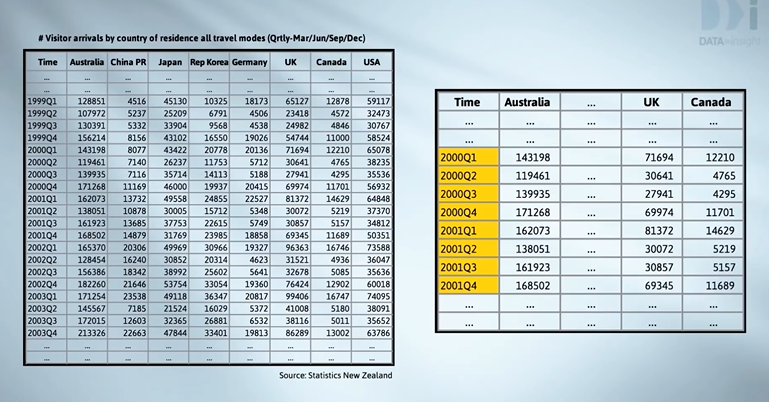
Here's a portion of a set of data on visitor arrivals to New Zealand. It's quarterly data, which means becasue the data is recorded four times a year covering periods of three months. Notice how the time variable is represented. With the year and then the quarter of the year (Q1 to Q4) for which the figures are given. Arrivals are reported separately for 8 countries. Data recorded over time like this is called time series data. The time format is the one used by statistics new zealand. Variants like this are used for statistical purposes around the world.
We will be introduced to plotting data against time and some patterns that can be revealed.
We will move on to estimating seasonal differences, forcasting and comparing related series. We will be dealing with only the single case in which each series will have a single observation point and our times are equally spaced.
Here's a portion of a set of data on visitor arrivals to New Zealand. It's quarterly data, which means becasue the data is recorded four times a year covering periods of three months. Notice how the time variable is represented. With the year and then the quarter of the year (Q1 to Q4) for which the figures are given. Arrivals are reported separately for 8 countries. Data recorded over time like this is called time series data. The time format is the one used by statistics new zealand. Variants like this are used for statistical purposes around the world.
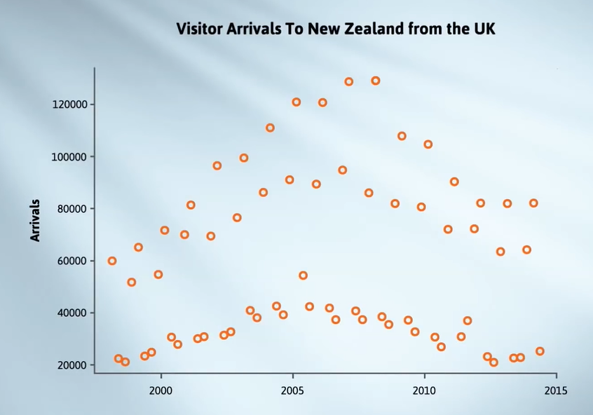
So what do we do with data like this? We could try a scatter plot with the following result. There are some patterns.We can see some bands going up and down. But people don't plot time series data like this.
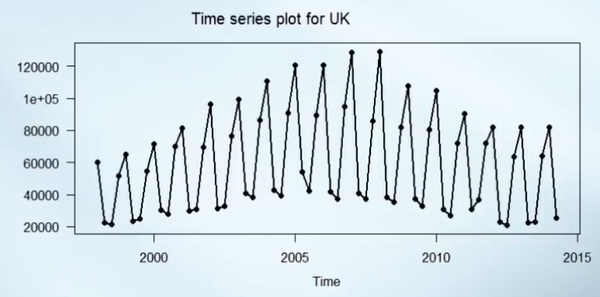
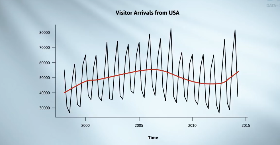
Typically the data is plotted against time and the points joined up by lines. The saw tooth pattern we couldn't see in the scatter plot jumps out at us as the points get connected up. The major things we see now are an overall trend and the saw teeth. Notice there is a basic pattern that repeats every year. These are called seasonal patterns.
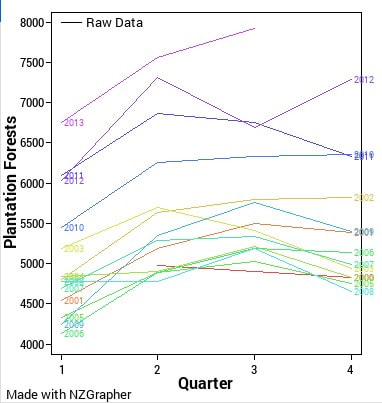
We can see the data better here where we have plotted the data against quarter with a separate line for each year. Every year the visitor numbers are biggest in the months Jan to Mar quarter (NZ summer months) and lowest in the Apr - Jun and Jul -Sep quarters, (NZ winter months). We might suspect that the Oct - Dec figures are high because in NZ december is a warm month and contains the Christmas holidays. The big months are Jan, Feb and Dec.
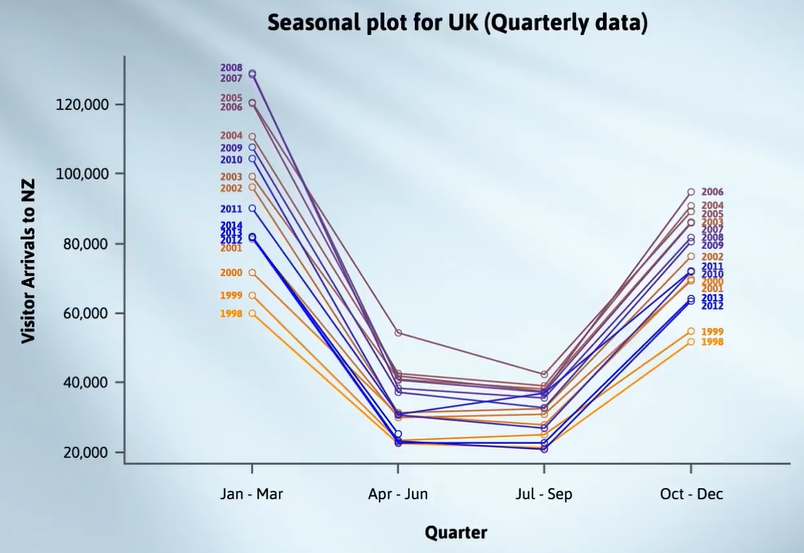
Seasonal patterns are common in time series data.
seasonal composition and forcasting
Looking at visitor arrivals from the USA.
Creating the seasonal plots.
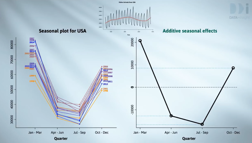
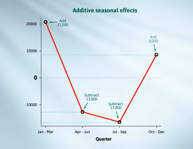
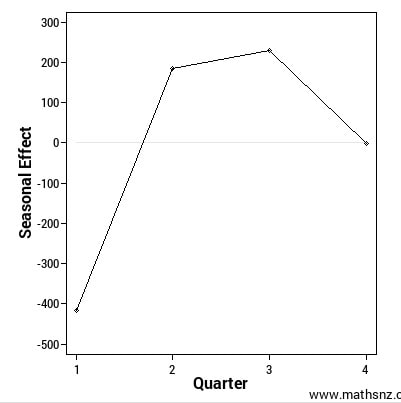
The average seasonal effect is shown in the right hand diagram. If seasonal effects are constant over time then looking below we can see that the Jan to Mar figures will be about 21000 visitors above what you would expect from the trend. The Apr to Jun figures are about 13000 visitors below. Jul to Sep is about 17000 below and Oct to Dec is about 8000 visitors above what you would expect from the trend.
using arctic sea ice as an example for decomposition.
Since you have a copy of the class exemplar for arctic sea ice, we will use that data set instead of the visitors to New Zealand data set. The data set is from NZGrapher and the method is exactly the same. The graphs for seasonal and residual are given below. (This is the oldest data set - not the three updated 2017 - 2019 datasets).
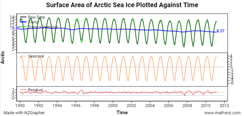
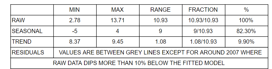
Firstly we construct a table that compares seasonal, trend and residuals as a percentage to the raw or real data. Raw or real data is the black line, green is the model that NZGrapher uses to construct its graph and the trend line is shown in blue.
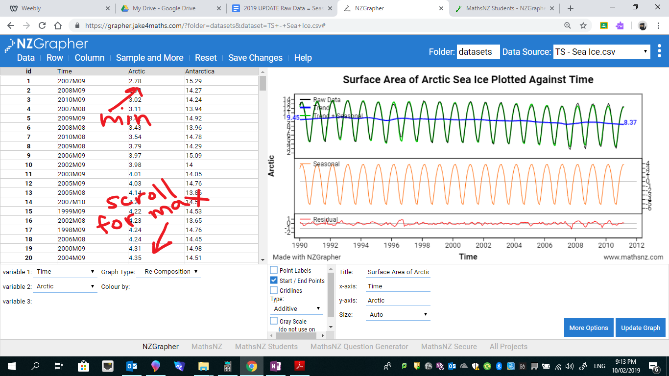
To find the min and max raw data values click on the "sample and more" menu, select sort and Arctic, as shown below.
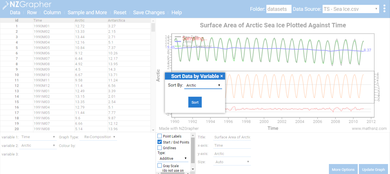
The following screen should appear. The minimum value is located at the top and you have to scroll down the list to obtain the maximum value. The difference or range is 10.93 This corresponds to 100%.
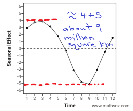
Next is seasonal as a percentage of raw data. This can be estimated by refering to the seasonal graph. The range is 9 million square km. As a percentage compared to the raw data this is
9/10.93 = 82%
This is the larger of the values and should make sense because the ice is increasing and decreasing mainly to the change in seasons.
9/10.93 = 82%
This is the larger of the values and should make sense because the ice is increasing and decreasing mainly to the change in seasons.
For the trend graph the start and end points can be obtained by checking the "start/end point" check box, 9.45 - 8.37 = giving a percentage of about 9.9% compared to the raw data. The trend is showing a gradual decline in sea ice area.
residuals graph
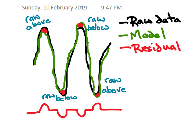
NZGrapher is doing some formulating behind the scenes. It is not just plotting the raw or real data only. Because one of the main uses for time series graphs is predicting future trends (forcasting), the residuals graph plays an important role in providing confidence in the model it uses. Residuals are the variation left over not explained by NZGraphers model for trend + seasonality. The residual graph shows the distance between the raw data (what actually happened) and NZGraphers fitted line (The model).
Residual line = 0 :The raw data is exactly the same as the fitted model (that would be nice!)
Residual line below zero: The raw data value is below the fitted model (model too high)
Residual line above zero: The raw data value is above the fitted model (model too low)
Here's another graphic to help explain this but remember not to get wound up about this technical detail. It's the overall concept that is required.
NZGrapher puts a limit line or 10% band on the residual graph. If the residual line exceeds the 10% line only a couple of times we can have confidence in the model. Any more than that, then our confidence decreases in proportion to the number of times it exceeds 10%. This is an estimation only.
So what is required in the report?
The downward trend contributes to about 9.9% of the total variation in the amount of Arctic sea ice present in millions of square km from Jan 1990 to Mar 2011. In comparison, the seasonal component contributes about 82.3% of the total variation in the series. This suggests that the stage (time) of the year has a greater influence on the amount of Arctic ice remaining. Looking at the residuals graph there is only one point where the raw data is more than 10% below the trend (fitted model). This occurred in Sept 2007 and may have been due to a usually hot summer. Based on the results of the residual graph I would be fairly confident about the model that NZGrapher is using for this data set.
The downward trend contributes to about 9.9% of the total variation in the amount of Arctic sea ice present in millions of square km from Jan 1990 to Mar 2011. In comparison, the seasonal component contributes about 82.3% of the total variation in the series. This suggests that the stage (time) of the year has a greater influence on the amount of Arctic ice remaining. Looking at the residuals graph there is only one point where the raw data is more than 10% below the trend (fitted model). This occurred in Sept 2007 and may have been due to a usually hot summer. Based on the results of the residual graph I would be fairly confident about the model that NZGrapher is using for this data set.
NZ FORESTRY EXAMPLE
intro
what do you want to find out?
what are you going to do?
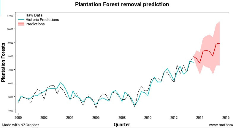
News reports have made me aware that New Zealand's construction industry is growing rapidly due to increased demand on housing. As a result, I believe the Forestry industry needs to be increasing its output from its plantation forests to meet this demand. (This work was done before the COVID 19 Epidemic and will be interesting to see how the data is affected in the future).
question
I want to investigate whether the logging of New Zealand plantation forests is increasing over the years and predict the amount of logging being carried over the next 2 years .
Variable 1) Quarter.
Time measurements are carried out quarterly i.e. three months per quarter and four quarters per year.
Variable 2) Plantation Forests.
This represents the volume of wood removed from different types of forests in New Zealand in millions of cubic meters.
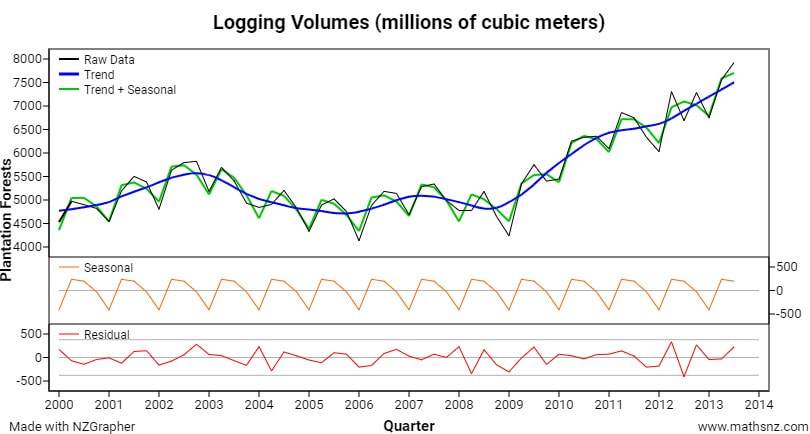
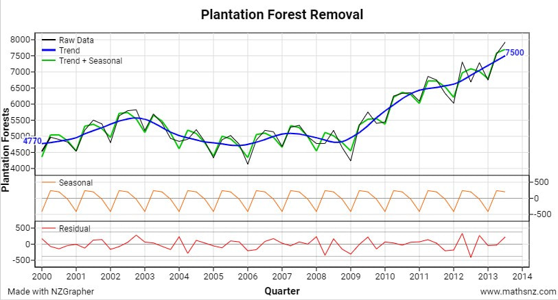
data
[This is where you reproduce the graphs from NZGrapher.]
|
|